Category Archives: in-focus

IN FOCUS: Making the Most of Your Microscope.

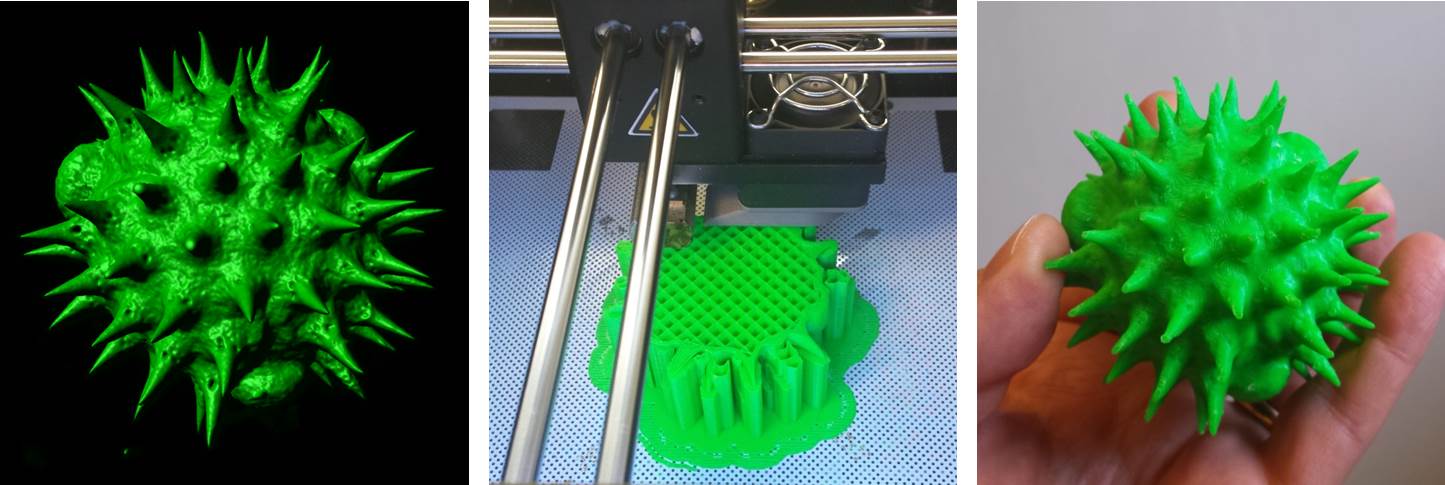
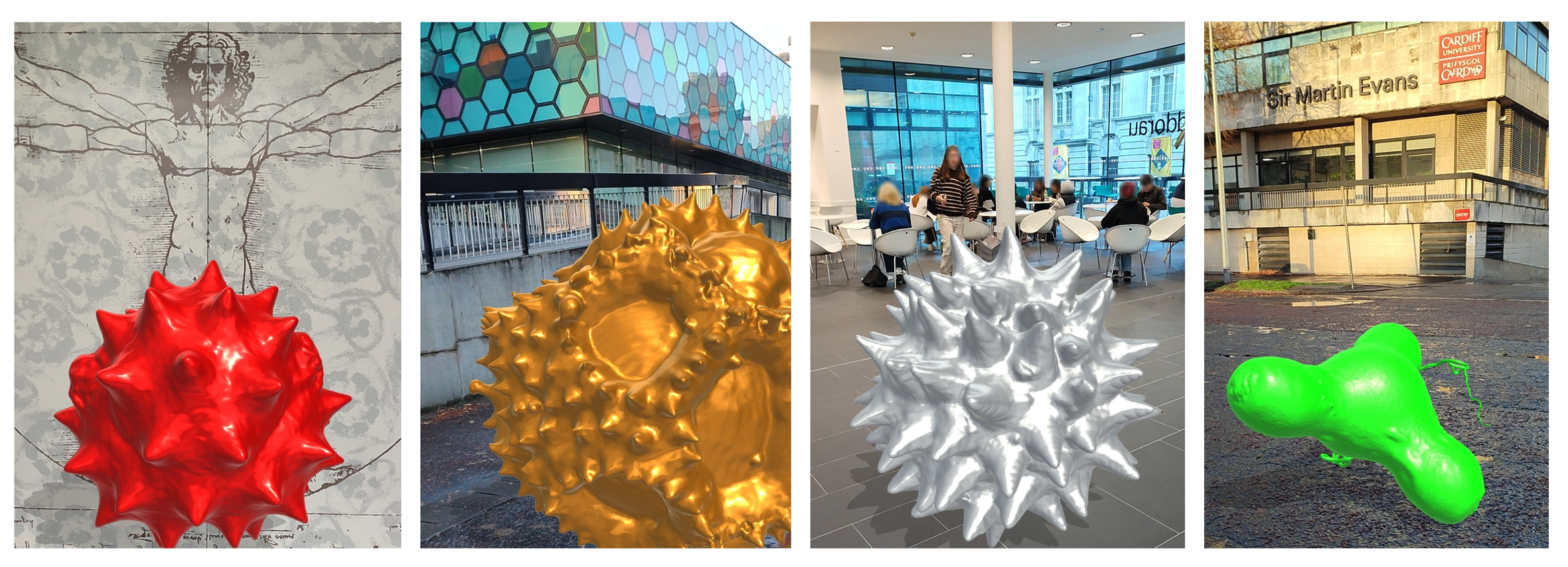
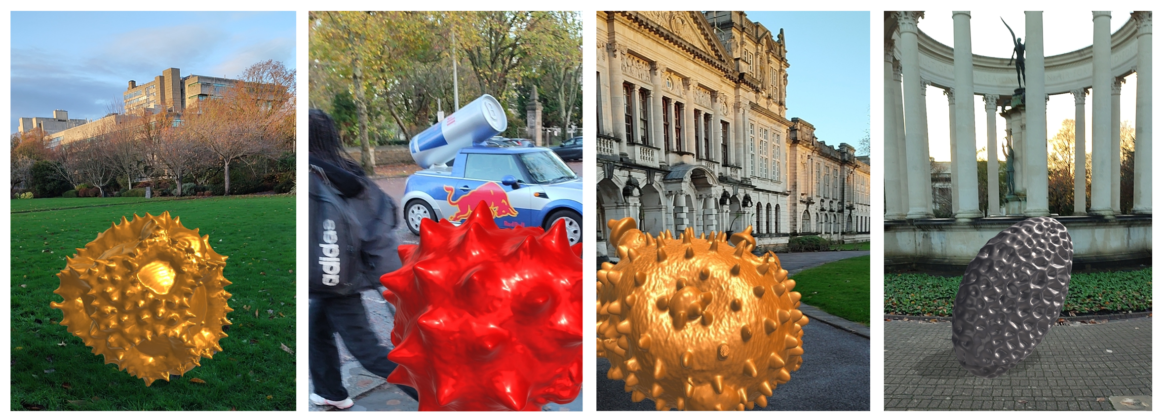
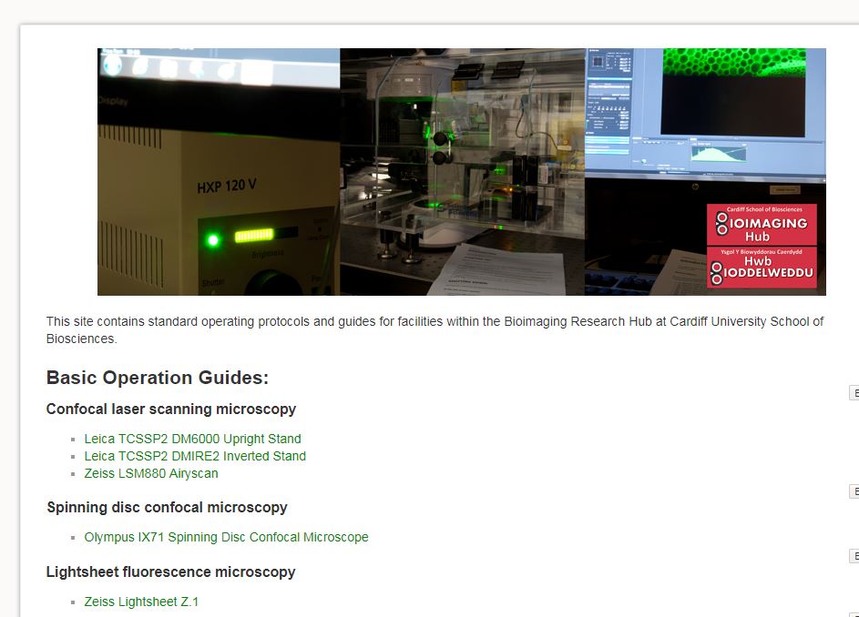
Above: A selection of stage plate inserts 3D printed by the Bioimaging Research Hub – links to resources in blog article below.

Hands up if your microscope is badly in need of upgrade or repair but your budget won’t stretch that far? Maybe a new focusing knob to replace the one that just broke off in your hand, or perhaps a new stage plate adapter, reflector cube or filter holder to increase your imaging options? Perhaps a C-mount or smartphone adaptor to give one of your old microscopes a new lease of life? Or even a sample holder or chamber for a bespoke imaging application? What the heck, let’s think big eh? How about a completely new modular microscope system with tile scanning capabilities?

Way too expensive, eh?… Well, imagine for a moment that you could just click a button (or a few buttons, at least) and make it so. If you haven’t yet realised, I’m talking about 3D printing in light microscopy and the life sciences – the subject of a very interesting paper that I recently came across – see below.

It’s safe to say that 3D printing is changing the way we do things in microscopy, now permitting low-cost upgrade, repair, or customisation of microscopes like never before. There are now a huge selection of 3D printable resources available through websites such as NIH3D, Thingiverse etc that can be used to modify your microscope system or to generate scientific apparatus or labware for upstream sample processing and preparation procedures.

So, to save you trawling through the 3D printing sites in order to identify the most useful designs to meet your histology and imaging needs we’ve done it for you and have curated a list of 3D printable resources which we hope you you’ll find useful (below).

AJH 25/05/2023

IN FOCUS: AR Palynology: Probing the Reality of Nature/Nature of Reality.

Above: Augmented reality visualisation of pollen grains 3D rendered in gigantic proportions. You wouldn’t want one of these getting stuck up your nose!

Back in 2015 we developed some novel methodology that allowed us to generate 3D printed models from confocal z-stacks of microscopic samples. At the time, we showcased the technique by making 3D prints of pollen grains from various plant species for use in science education and outreach activities, musing that a physical, tangible model would allow improved 3D conceptualization of these microscopic structures – original blog article here. The work generated a fair amount of interest and resulted in requests for 3D printed models of pollen grains from far and wide (e.g., the Smithsonian National Museum of Natural History in the US, the UK Met Office, National Botanical Garden of Wales etc). Following publication of our methodology in 2017 other researchers soon followed suit, creating their own 3D printed models from confocal datasets utilizing methods similar to ours. By this time, we had turned our attention to virtual reality (VR) as a tool to experience/manipulate microscopic objects, as well as larger more complex biological models in virtual space – something we saw as a logical evolution of the 3D learning experience. You can read more about this in a separate blog and see the progress we made in developing the resource via a short video on our YouTube site.

Fast-forward to present, a global pandemic, accelerating environmental change, and a cost-of-living crisis – the economic fallout from COVID, the folly of Brexit, a war in Ukraine, and gross government incompetence. To borrow a quote from a certain Vladimir Ilyich Ulyanov, there are decades where nothing happens, and there are weeks where decades happen. Well, quite!

But what of the 3D pollen models? Well, for one, coronaphobia has meant that people are less inclined these days to be handling and passing around shared resources such as plastic pollen models or VR headsets at risk of spreading/contracting germs. Moreover, plastic is increasingly being viewed negatively due to the environmental damage caused by plastics and ‘frivolous’ 3D printing could be seen as increasing the existing plastic problem. Lastly, with the cost-of-living crisis/looming recession, it would seem that no one can afford to do anything other than feed themselves and try to keep warm these days, let alone commission 3D pollen prints from the Bioimaging Hub – particularly since there’s now a growing number of pollen models available through 3D printing sites such as Sketchfab etc. And so, with these concerns in mind, we’ve donned our thinking caps and come up with a plan to address the prevailing zeitgeist.

Firstly, we’ve decided to make our entire repository of 3D pollen models publicly available, free of charge, under a Creative Commons CC-NY-NC licence via the newly developed NIH3D website (formerly the NIH3D print exchange) which is a leading community-driven portal for sharing and downloading bioscientific content for 3D printing and interactive 3D visualization. Under the terms of our licence, the models can be used, shared, or modified for non-commercial purposes, as long as the creator(s) are properly credited. To date, we’ve made available 3D models of seventy distinct species of pollen grains and spores through the Bioimaging Hub’s new NIH 3D profile page which have now been curated into a special collection, the 3D Pollen Library We have also included all source data (confocal z-stack files in Carl Zeiss Image .czi file format). To the best of our knowledge, this represents the largest single collection of 3D pollen files available online and the plan is to add more models plus supporting data in future. For cross-referencing, relevant links have been included to major palynological databases, PalDat and the Global Pollen project, and, of course, Wikipedia – the fount of all knowledge : ) We’ve also showcased a small selection of our pollen models on the Bioimaging Hub’s Sketchfab site – these can’t be downloaded directly, however you can manipulate the models on screen and view them in VR – further information here.

Secondly, we’ve been experimenting with augmented reality (AR) as a tool to allow visualization and exploration of our 3D models in real-world environments. The beauty of AR, of course, is that it doesn’t require a headset, just a smartphone or tablet which are now more ubiquitous than ever. Thus, a 3D model in the relevant file format (usually .glb or .gltf) can be downloaded directly to an individual’s smartphone or tablet and, using appropriate AR software, seamlessly integrated with real time digital information from the camera for display on the touchscreen. This allows users to personally experience a real environment with generated perceptual information overlaid upon it. Within the AR environment, the models can be scaled up or down, freely moved and rotated via the touchscreen, or circumnavigated and explored both externally and internally via directional information from the device’s sensors, à la Pokemon-GO. This allows for a highly realistic and immersive interactive experience (different from the artificial environments of VR) thus facilitating 3D conceptualization of the embedded model. Furthermore, freed from the physical encumbrance of a VR headset, the user is less likely to blunder into office furniture, moving traffic etc or experience the nausea, headaches and dizziness of VR-associated cybersickness.

So how does one view our 3D pollen models in AR? Well, it’s quite straightforward really, but to make things even easier I’ve put together a set of instructions (below) that should get you up and running in next to no time:

Install a free AR app on your mobile device (smartphone or tablet) from the Google Play or Apple App stores that handles .glb (GL transmission format binary) files – this is the common standard file format for AR/VR visualisation. There are quite a lot of AR apps to choose from and we’ve only tested the NeoSpace AR app on android devices but this seems to work quite well.
Go to the Bioimaging Hub’s NIH 3D webpage – link here – select a 3D pollen model, and then click on the DOWNLOAD option. You will then see a list of the files that we’ve made available for download (refer to screenshot below). These include:

.glb file format for AR/VR applications (available as both zipped and unzipped files).
.stl (stereolithography, .wrl (‘worlds’ virtual reality modelling) and x3d file formats for 3D printing applications.
source confocal data in .czi (Carl Zeiss Image) file format (zipped file).

For AR viewing, download the .glb file to your mobile device (if zipped then extract the compressed file).
Open the .glb file in the AR viewer app and follow the on-screen instructions. Initially you’ll have to scan your environment with the camera on your smartphone/tablet so that the app can identify a flat surface in order to place the 3D model into your display.

If you’ve done it correctly then you should now be able to view any of our 3D pollen models in whatever context your imagination, mobile device and AR app allows. Below are some examples of the type of AR imagery that we’ve generated using a free android AR app.

Above: Video sequence captured from an android smartphone running the free AR app, NeoSpace. The 3D pollen model can be zoomed, freely moved and rotated via touchscreen and also circumnavigated and explored both externally and internally via directional information from the device’s sensors.

Above: Attack of the giant pollen grains! Photo-realistic AR imagery generated using an android smartphone and the NeoSpace AR app.

We’d love to get some feedback with photos or videos showing how you have used our pollen models for 3D printing, or AR/VR applications in science education and outreach. Please keep us updated via our twitter account @cubioimaginghub. Best of luck!

AJH, November, 2022 (updated March 2023).

Further reading:

Perry, I., Szeto, J-Y., Isaacs, M.D., Gealy, E.C., Rose, R., Scofield, S., Watson, P.D., Hayes, A.J. (2017) Production of 3D printed scale models from microscope volume datasets for use in STEM education. EMS Engineering Science Journal. 1 (1): 002
IN FOCUS: Bigging it up: 3D printing to change the shape of microscopy (February, 2016).
IN FOCUS: Development of a 3D printed pollen reference collection (August, 2016)
IN FOCUS: 3D Pollen prints not to be sniffed at: printing pollen for the met office (July, 2017).
IN FOCUS: Immersive Microscopy: 3D visualisation and manipulation of microscopic samples through virtual reality (February, 2019)
IN FOCUS: Plastic fantastic: making pollen models for the National Botanic Garden of Wales.(October, 2019)
IN FOCUS: AR Palynology: probing the reality of nature/nature of reality (November, 2022)

IN FOCUS: Standard Operation Procedures (SOP) Repository.

Above: A screenshot of the Bioimaging Hub’s SOP repository

If you wasn’t already aware of the Bioimaging Hub’s SOP repository (N.B. there are shortcuts set up on all of the networked PCs within the facility), then please take a look at your earliest convenience. The database was set up as a wiki to provide Hub users with up to date protocols and tutorials for all of our imaging systems, experimental guidelines for sample preparation, health and safety information in a variety of multimedia formats in one convenient and easily accessible location. It’s still work in progress and we would welcome any feedback on how the resource could be further developed or improved.

AJH 7.1.19

IN-FOCUS: Making Imaris a Bit(plane) Faster

Most of the work of the Bioimaging Hub is concentrated on acquiring images – choosing the right equipment, optimising settings, advising about sample prep, etc. We do, however, have a few systems dedicated to analysing images too. We’ve got a system running Arivis Vision4D which specialises in extremely large datasets, such as Lightsheet data, as well as a system running Bitplane Imaris. We’ve had Imaris for longer and so it’s seen a lot more use. This was recently updated with a Filament Tracer module for analysing neuronal processes. Shortly after this upgrade was added we experienced a severe slowdown in the software. It would take over a minute to go from the ‘Surpass’ view, where images are analysed, to the ‘Arena’ view, where files are organised. The information for the files in Arena is stored in a database and we suspected that the database was at fault.

Imaris hanging when switching from Surpass to Arena. It would do this for about 65 seconds every time a change was made.

A call with Imaris technical support was arranged and the software examined. There were no apparent errors in any of the logs and the database was functioning as it should. The only advice available was to thin down the number of entries in the database – we were told it had nearly 240,000 entries which, even accounting for metadata, seemed vastly excessive for the number of files in Arena.

Complete database dump of nearly 240,000 entries.

I decided to try to trim the database.

My first thought was the Filament Tracer module was generating a large amount of statistics and these were being stored in the database. A couple of users had been experiencing crashes when accessing these statistics so it was possible that slow database responses were bringing the software down. I backed up all datasets which used the Filament Tracer (a process far more laborious than it should be) and deleted them all from Arena. This dropped the database access time from 65 seconds to 60. Not that much of a result.

My next thought was that the co-ordinates for the vertices of surface renders might have been clogging up the database. We’ve generated quite a lot of 3D models of pollen grains and cells so this was potentially a lot of data. I went through the same laborious process of exporting all these datasets and deleted them. Again, little improvement.

I decided I needed to look at the database directly. The underlying database runs on PostgreSQL as part of the BisQue bioimaging package. Using the pgAdmin tool I began to browse the database to see where the data was held and how it was organised.

Structure of the underlying database.

I couldn’t find any trace of it so I exported the entire thing as a text file and loaded it into NotePad++. As Imaris technical support had told us, it was enormous – 55MB of text. Scanning the file, eventually I found that practically all the data was held in a database table named ‘taggable’. I’d skipped over this at first as the name was so nondescript.

Using Notepad++ to check a database dump and find where the data is stored – the table named ‘taggable’.

Once I knew all the data I needed was in this table I began to examine it. The first thing that jumped out at me was the huge number of entries in the database relating to datasets from our Leica confocal system. This system stores its data as a series of tif images, one per channel, one per z-position for z-stacks. Every single one of these files had its own database entry as a dependency for a ‘resource_parent_id’.

Database entries for Leica datasets. One record per channel, per z-position which becomes a huge number of entries.

A lot of old Leica datasets had been loaded into Arena recently to see if any new information could be extracted from them and this had massively inflated the size of the database. I exported all these datasets as new Imaris .ims files and deleted them from Arena. This reduced the number of database entries from just under 240,000 to just over 16,000. As a result the database access time dropped to about 18 seconds. Much more manageable but still a bit slow.

Looking at the database entries again, I could see that there were still lots of entries relating to Leica datasets. I went back to look at Arena but there was no sign of them. These were orphaned entries relating to non-existent data. As it was impossible to delete them from Arena, I identified all of their resource_parent_id numbers and used pgAdmin to delete them

Manually deleting orphaned database entries.

It then occurred to me that the indexes for the database were probably totally out of date so my final task to optimise things was the rebuild all of the indexes in pgAdmin

Rebuilding the table indexes.

All of these steps got the database access time down to 3 seconds – quite a bit improvement on the original 65 seconds! Importing some of the exported datasets as Imaris .ims files slowed it back down to about 10 seconds so it’s apparent that the database scales very poorly. Still a lot better than when the Leica datasets were numerous separate files though. It looks to me that the database design favours flexibility over scaling which ends up being not very useful if you want to use it to organise a reasonable amount of imaging data.

So if you’ve got Imaris database lag there’s a few things you can try. The main improvement was to make sure your datasets are represented by single files, either by exporting them as Imaris .ims files or converting them to something like OME-TIFF first.

—
Marc Isaacs, Bioimaging Technician

IN FOCUS: Cutting Through the Fog: Reducing Background Autofluorescence in Microscopy.

Above: Autofluorescence from mixed connective tissues imaged by confocal microscopy (left). The autofluorescent emissions can be spectrally-resolved through wavelength scanning (right). Excitation at 488nm.

Whilst autofluorescence from endogenous fluorophores can reveal much about the biochemical composition of a sample, it can also hamper the microscopic detection of targeted fluorochromes if they emit light at the same wavelengths as endogenous fluors. Indeed, without proper controls, complex background autofluorescence can lead to misinterpretation of image data and generation of false positive results.

Autofluorescence derives from multiple sources within the sample – the main culprits are NADH and NADPH, lipofuscins, flavins, elastin and collagen (and lignin and chlorophyll in plants). The excitation and emission ranges of the worst offenders have been shown below. It follows that tissues with high collagen and elastin contents, e.g. skin, tendon and cartilage, autofluoresce very brightly; as do tissues that are rich in metabolic breakdown products such as lipofuscin, e.g. liver, spleen etc.

Adding to the problem is the effect of chemical fixatives (e.g. formalin, glutaraldehyde etc) and solvents used to preserve tissue architecture for microscopy: the cross-linkages generated by these chemicals increase autofluorescence, which can be worsened further by long-term storage of the fixed processed tissues.

So, dear reader, here’s some simple advice on steps that you can take to address this common problem:

1. Include an unlabelled control to evaluate the level of autofluorescence within your sample.

Observation of unlabelled samples through RGB fluorescent filters (note their transmission characteristics) will help identify where in the visible spectrum the autofluorescent signal is brightest.
Spectral (lambda, wavelength) scanning will allow you to precisely identify the fluorescent emission spectra from endogenous fluorochromes and can help separate their emissions from those of your fluorochrome (see above figure).

2. Select fluorochromes that are outside the range of the autofluorescence.

If the autofluorescence signal is high in the blue, then move into the green; if it’s high in the green, move into the red – or better still, the far red (if your system can detect in this range).
Use modern fluorescent probes (e.g. Alexa Fluor, Dylight, or Atto range) instead of first generation fluorochromes. They are brighter, more photo-stable and have narrower excitation and emission bands. They are also available in variants that span the near UV, visible and far red range of the spectrum, affording you plenty of choice.

3. Use a microscope with filters optimised for your choice of fluorochromes.

Band-pass filters which collect emissions within a specific range may be more useful than long-pass filter sets which collect all emissions past a certain wavelength. The narrower the range of the band-pass filter, then the better it can separate fluorophores with close emission spectra.

4. If the autofluorescence is unevenly distributed within your sample, use targeted microscopy to avoid it.

5. If you can’t avoid the autofluorescence, then take measures to remove or reduce it.

Analyse the pixel intensity distribution within your image and try thresholding out the lower intensity autofluorescence signal.
Pre-bleach your samples in a light box using a high intensity illumination source prior to fluorescent labelling (see below reference)
Treat samples with a chemical reagent (e.g. sodium borohydride, Sudan black B, ammonium ethanol etc) to reduce background autofluorescence (see below reference)

6. If all else fails, consider the following:

use cryoprocessed material as an alternative to chemical fixation and paraffin wax processing.
avoid long term storage of material/archival tissue samples.
try a different detection modality (e.g. immunoperoxidase instead of immunofluorescence)

AJH

IN-FOCUS: Better To Burn Bright Than To Fade Away: Reducing Photo-bleaching in Fluorescence Microscopy.

Above: Photo-bleaching (fading) occurs when a fluorochrome permanently loses the ability to fluoresce due to photon-induced chemical damage and covalent modification.

Hands up if you’ve spent hours preparing a sample for fluorescence microscopy only to see the signal disappear before your eyes upon excitation? Frustrating eh (unless, of course, FRAP is your objective)? Well here’s some simple and sound advice on how you can minimise photo-bleaching and get the best out of your samples under the fluorescence microscope.

1. Visualise your samples immediately after fluorescent labelling – this is when they are at their brightest.

If this is not possible then loosely wrap your samples in aluminium foil and keep them in the dark at 4oC until you get the opportunity to image them.

2. Minimise their exposure to light in order to reduce photo-bleaching.

visualise your samples under low light conditions.
use transmitted light to find a region of interest (ROI) and then switch to epifluorescence observation – avoid dwelling too long on the ROI.
step down the intensity level of excitation light or insert a neutral density filter into the light path.
set up imaging parameters on a neighbouring region and then return to the ROI for image capture.
use image binning to reduce exposure time.
use the microscope shutter to switch off the light source between images.
create a photo-bleach curve from a timed series of images. This can be used to normalise for loss of fluorescence intensity.

3. Switch to a mounting medium with anti-fade protection e.g. Vectashield, Prolong Gold/Diamond, SlowFade Gold/Diamond. These work by reducing the oxygen available for photo-oxidation reactions, thus reducing photo-bleaching. N.B. Many of these are available with a nuclear counterstain (e.g. Dapi) included in the formulation. Alternatively, make your own anti-fade reagent (instructions below).

4. Switch to brighter, more photo-stable fluorochromes. First generation fluorochromes such as FITC and TRITC photo-bleach readily (and are pH sensitive) thus should be replaced with modern dyes such as the Alexa Fluor, Dylight, or Atto range of fluorochromes, which are much brighter and far more photo-stable.

Good luck!

AJH

IN-FOCUS: Development of a 3D printed pollen reference collection.

Above: surface-rendered confocal reconstructions of pollen samples (left) and their corresponding 3D printed models (right).

Isn’t the World Wide Web a wonderful thing? Not so long ago I wrote a short blog explaining how we had developed methodology to convert volume datasets from the confocal microscope into 3D printed models – perfect solid scale replicas of samples the size of a pollen grain etc. Well, shortly afterwards I received an email from someone who had not only read the blog but, serendipitously, wanted to do this very thing! What is more, she was located not a million miles away: in fact, little more than 400 yards down the road from us, working as a researcher within Cardiff University’s School of History, Archeology & Religion. Please excuse the pun, but it really is a small world!

Rhiannon Philp is an archaeologist – or palynologist to be precise – someone who studies ancient pollen grains and spores found at archaeological sites. Pollen extracted from archeological digs can be used for radiocarbon dating and for studying past climates and environments by identifying plants growing at the time. Rhiannon is using this information to develop an understanding of prehistoric sea level changes in South Wales as part of the Changing Tides Project.

Rhiannon asked if we could generate a reference collection of 3D pollen prints that could be used for teaching and outreach activities as part of a new Archaeology engagement project called Footprints In Time. Indeed, some of her pollen samples were from sites containing both human and animal footprints made over 5000 years ago!

You can see some of our results above: on the left are the surface-rendered confocal volume reconstructions and, on the right, their corresponding 3D printed facsimiles – courtesy of the BIOSI 3D printing facility.

If you’re at the National Eisteddfod in Abergavenny this week (29th July – 6th August), then please pop by to see Rhiannon’s stall within the Cardiff University tent – all of the models will be on display there, together with a lot more. Any further interest, then please get in touch.

AJH

IN-FOCUS: Bigging it up: 3D printing to change the shape of microscopy.

Imagine being able to generate a highly accurate, solid scale replica of the sample that you are visualising down the microscope; a perfectly-rendered pollen grain, or blood cell, or microscopic organism, but big enough to hold and examine in your hand. It would allow much better 3D conceptualisation of the sample, particularly for blind or visually-impaired individuals, and would have enormous utility in teaching and in engagement activities, and what researcher wouldn’t want a tangible, physical embodiment of their research to help explain their work (and impress their colleagues) at scientific meetings? Sounds like the stuff of science fiction doesn’t it? Well, not any more. Thanks to 3D printing technology (and the help of Dr Simon Scofield‘s lab) we have started taking volume datasets from the confocal microscope out of the virtual world and making them a reality. If you would be interested in generating a highly accurate scale model of your favourite biological sample (or would simply like to handle a giant pollen grain!) then please feel free to get in touch.

AJH

IN-FOCUS: Microscopy on the move. A round-up of the best microscopy apps for mobile devices.

Here’s a quick round up of some useful imaging applications for portable Android and Apple devices.

Cell Imaging HD. Molecular Probes cell imaging guide with protocols. This mobile app is designed to help you find fluorescent dyes, reagents and protocols for cell biology related fluorescence microscopy applications.
- Google Play Store (Android mobile devices)
- iTunes App Store (Apple mobile devices)

Fluorescence SpectraViewer. Plot and compare spectra, check the spectral compatibility for many fluorophores and email the configuration to yourself or to others in the lab in a clear printable format.
- Google Play Store (Android mobile devices)
- iTunes App Store (Apple mobile devices)

Leica DMShare. Allows wireless transfer of microscopy images from the latest Leica camera systems to one or more Android devices.
- Google Play Store (Android mobile devices)
- iTunes App Store (Apple mobile devices)

Microscopy and Analysis journal. The leading international magazine for microscopists. Loads of interesting articles, features and news on microscopy and imaging.
- Google Play Store (Android mobile devices)
- iTunes App Store (Apple mobile devices)

Smart Histology. Microscope emulation that allows zooming and panning of over 100-histological tissues. A free LITE version is also available so that you can try before you buy.
- Google Play Store (Android mobile devices)
- iTunes App Store (Apple mobile devices)

Molecular Probes 3D Cell App. Learn about the cell and all its structures in 3D on Apple portable devices. Enjoy the ability to rotate the cell 360 degrees and zoom in on any cell structure.

Zeiss microscopy apps. Compendium of Zeiss microscopy apps specifically for Apple portable devices (Light Lab, Zen Browser, Zen remote, Labscope, Matscope)

If you wish to use your smartphone camera as a rudimentary digital magnifier just search ‘microscope’ in either the Google Play or iTunes App stores – there’s loads to choose from. Instructions available here showing how to build a perspex support stage with transmitted light illumination for your smartphone. If you want anything more sophisticated, take a look at this.

AJH

IN-FOCUS: Microscopy and Analysis Journal: A Useful Resource for Microscopists.

I can see why Microscopy and Analysis is the leading international journal for microscopists – it’s chock-full of interesting articles, features and news on all things related to microscopy and imaging. More to the point, it’s free to individuals who purchase, specify or approve microscopical, analytical and or/imaging equipment at their place of work. The journal is published six times per year, in January, March, May, July, September, and November. There are also several supplements published periodically, which include publications devoted to special events, trade shows and specific areas of microscopy and imaging. The journal is available in print, or can be viewed online in an interactive format, or via a downloadable app. We also have lots and lots of back issues available within the Bioimaging Unit, which you are welcome to peruse on your next visit!

AJH

Bioimaging Hub News

News from the Bioimaging Research Hub in the School of Biosciences, Cardiff University.