NEWS: State of the Art: An Update.

Above: Plant parts x4 . Biological pop-art on the ‘Warhols’ of the Bioimaging hub. Slide scanned images of plant tissues (various species; transverse sections) courtesy of Dr Tony Hayes, pop-art montage by Marc Isaacs.

The eagle-eyed amongst you may have noticed that the main corridor within the Bioimaging Research Hub is looking a little nattier these days. We thought it required some brightening up and so have started to adorn its walls with some nice, new A0-sized foamex prints of microscopical images that we’ve generated in-house on the Hub’s microscope systems. We’ve tried to select images that showcase the beauty of the unseen microscopic world which reflect the art in science, or ‘SciArt’ as it is known. We hope the images stimulate interest and highlight the state-of-the-art research and facilities within Cardiff School of Biosciences. No prizes for spotting the artistic influences on some of our ‘works’ : )

AJH

Further reading

Sleigh & Craske (2017) Art and science in the UK: a brief history and critical reflection. Interdisciplinary Science Reviews. 42:4, 313-330.

IN FOCUS: Plastic Fantastic – Making Pollen Models for The National Botanic Garden of Wales.

The Bioimaging research hub does a nice sideline 3D printing scale replicas of biological samples for use in science engagement and teaching. These can be made from the smallest of microscopic samples imaged via optical sectioning microscopy (i.e., confocal or lightsheet) or from large anatomical samples imaged via 3D photogrammetry or from 3D scanning techniques. I’ve posted a few blogs on this site in the past describing 3D pollen models that we’ve made for various research groups within Cardiff University (e.g. for the ‘Footprints in time’ and ‘PharmaBees’ projects) and for a growing number of external organisations within the UK and abroad (e.g. the Met office, the Smithsonian institute etc).

Recently, we were approached by the National Botanic Gardens of Wales (NBGW) to generate 3D models of twenty different species of pollen grains identified in honey by Dr Natasha De Vere’s research group for their science outreach and engagement programme. Natasha is the head of science at the NBGW and is using cutting edge DNA bar coding technology to understand pollinator foraging preferences. This research is providing amazing insights into the selective range of plant species that important pollinating insects such as bees visit when foraging (you can read more about this fascinating work here and in the reference below).

To generate the 3D prints we first needed pollen samples from each of the respective plant species – you’d be forgiven if you thought the National Botanic Gardens could provide these ‘off the shelf’ : ) Coming from a zoological background, my botany field skills are best described as rudimentary. So, equipped with my smartphone, a plant identifier app that I downloaded from the Google Play store, and some zip-lock sample bags, I embarked upon a ‘Pokemon-go style’ palynological quest (‘gotta catch ’em all’) that took me to the local parks, woodlands, river embankments, country lanes and coastlines and even garden centres of South Wales.

After some effort, I managed to identify and collect all of the pollen species on the wish list. I then began to image representative grains from each species using the Hub’s Zeiss LSM880 Airyscan confocal microscope. Individual grains were optically sectioned through their volume, 3D reconstructed and then output in a file format for 3D printing on our Ultimaker 3D printer (method described in reference below).

The finished 3D pollen models are shown in the photograph above – each model is approximately 15cm in diameter (i.e., enlarged by a factor of approximately x400 relative to the original pollen grain). The models will be on display at the Growing the Future stand at this year’s Royal Welsh show (20-23rd July, 2019) and also at the Pollinator festival at the National Botanical Gardens of Wales (24-26th August, 2019).

AJH

Further Reading

Hawkins, J., de Vere, N., Griffith, A., Ford, C.R., Allainguillaume, J., Hegarty, M.J., Baillie, L., Adams-Groom, B. (2015) Using DNA metabarcoding to identify the floral composition of honey: a new tool for investigating honey bee foraging preferences. PLoS ONE 10 (8): e0134735. https://doi.org/10.1371/journal.pone.0134735.

Perry, I., Szeto, J-Y., Isaacs, M.D., Gealy, E.C., Rose, R., Scofield, S., Watson, P.D., Hayes, A.J. (2017) Production of 3D printed scale models from microscope volume datasets for use in STEM educationEMS Engineering Science Journal1 (1): 002.

Contributors

Sample collection and preparation, confocal microscopy, 3D reconstruction and file conversions by Dr Tony Hayes; 3D printing by Dr Pete Watson; Photography by Marc Isaacs.

CORE EQUIPMENT: Widefield Microscope Upgrades.

The Bioimaging Hub’s conventional widefield microscope systems have recently received some performance upgrades. Details of upgrades below:

N.B. All of the above systems are now networked via 1GB desktop switches. Up-to-date standard operating procedures and risk assessments for each system are available through the Bioimaging hub’s online SOP repository via their desktop folders (‘Read me before use’). See a member of staff for further details.

AJH

IN FOCUS: Winging It In Paleobiology: Strange Tails from a Strange Time.

Above: Some of the exhibits on display, including the Meganeura model made by the Bioimaging Hub, at ‘The Fossil Swamp’ exhibition at Cardiff Museum.

How do you make a dragon-fly (ask it nicely, I suppose)? Well, this was the question we were asking ourselves a few weeks ago after an email enquiry from Dr Trevor Bailey of the National Museum of Wales. Trevor is one of the museum’s senior paleontologists and is involved in curating many of the museum’s public exhibitions and programmes involving fossils and prehistoric life (You can read more via his profile page here).

Trevor had contacted us to enquire whether we might be able to help with a forthcoming exhibition at the museum, called ‘The Fossil Swamp‘, by making a scale replica model of an extinct insect species similar in appearance to a modern dragon fly (it’s actually classed as a Griffin fly), but with one big difference (and I mean BIG): its size. How big I hear you say? Well, to give you an idea of its sizeable dimensions, the wingspan of Meganeura was approximately 0.7 metres long (i.e. roughly the same wing span of a large, adult sparrow hawk)! Indeed, this is how the insect came to earn its rather ominous sounding moniker: ‘mega-neura’ means ‘large-nerved’, referring to the network of large veins supporting the insects enormous wings (Brongniart, 1893)

In fact, Meganeura monyii is one of the largest known flying insect species ever to grace planet earth. It lived more than 300 million years ago, in the carboniferous period where the atmospheric oxygen concentration of air was much higher than that of today (around 35% then, instead of 21% now) which, it is thought, allowed the insects of that period to grow to enormous proportions (insects breathe through small holes, or ‘spiracles’ in their body walls connected to branched air tubes called ‘tracheoles’ which convey oxygen to their internal tissues). Furthermore, at the time Meganeura was buzzing about, bugging the primitive lifeforms of the day, there were no other aerial vertebrate predators around (in fact, birds arrived to the table 75 million years later) so it could pretty much act with total impunity!

So Trevor supplied us with a digital model of the insect for 3D printing, together with the desired dimensions, based on recorded fossil evidence (Brongniart, 1893). Interestingly, the digital mesh was actually created as a component of a carboniferous forest simulation  by a colleague of his in Germany  (link here).  In order for us to 3D print Meganeura’s body to scale using our Ultimaker 3 extended 3D printer, we had to fabricate the head and thorax separately to the abdomen and then re-attach these after removal of their supporting scaffolds. We printed these using polylactic acid (PLA) filament at an intermediate print resolution. The first attempt looked okay, but the finished model was rather blocky in appearance, so we smoothed the digital mesh and then reprinted at a higher resolution with much better results.

1-2 digital reconstructions of Meganeura monyii; 3-5 3D prints of the separate body sections; 6 Support scaffolds removed and body sections reunited – note block appearance of model. The digital mesh was filtered and the model reprinted with much better results (see below).

The next challenge was those huge wings. I downloaded .png image files of the venation patterns recorded by Brogniart (1893) here. However they were simply too large to 3D print at the desired thickness (and believe us, we tried) so a different approach was necessary. Each wing was laser printed onto a separate sheet of acetate. These were then cut out and laminated – the composite structure increasing the rigidity of the wing but still allowing realistic flexion. To attach the wings to the thorax, I drilled holes through adjacent thoracic segments and fed lengths of wire through the holes to support the leading edge of each wing pair. The wire was then bonded in place to prevent any lateral displacement.

7 Wing venation pattern after Brogniart (1893) downloaded from the web; 8: wings laser printed to scale on acetate and laminated; 9 laminated wings cut to final shape.

Next up was the paint job, which became a labour of love (and exercise in mindfulness) in my spare time! Now, unfortunately, no one knows what colours or patterns adorned the body surface of Meganeura as the fossil evidence is all black and white. Artist’s impressions are therefore based loosely on modern equivalents (e.g dragonflies, damsel flies etc), or have just been made up to make the insect look as fearsome as possible – it was a carnivorous predator after all! So after a few Google image searches, just to get some ideas, I finally went with a black and yellow/orange colour scheme with iridescent bronze eyes (with artistic input from Trevor and my daughters). I used acrylic paints, purchased cheaply from The Works, which gave good adhesion and cover without the necessity of a primer coat. Fine detail was added under magnified optics.

10 Smoothed model with base coat of acrylic. Wires have been inserted through thoracic segments to support leading edge of wing pairs; 11-13 Model has been painted and the first pair of wings are awaiting attachment.

When the model was fully painted we attached the wings to the wire frames using extra strong clear sellotape before taking it over to Alexandra Gardens, opposite the School of Biosciences, for some wildlife photography, doing our best not to frighten the native fauna (or general public)!

14-15 The finished Meganeura model – a ferocious looking beast!
16-17 …and doing its best to blend in with the local flora!

The model will be on display as part of the Fossil Swamp exhibition in the National Museum of Wales at Cardiff from 18th May, 2019 to 17th May, 2020 along with lots of other amazing artefacts from the carboniferous period. Please go along to visit – it promises to be a fantastic family day out.

AJH

Further reading

  • Brongniart (1893) Recherches pour servir á l’histoire des insectes fossiles des temps primaires : procédées d’une étude sur la nervation des ailes des insectes (Research to serve the history of fossil insects of the early ages : preceded by a study on the wing venation of insects).

Contributors

Digital mesh of Meganeura monyii was taken from the Carboniferous forest simulation, page author and domain holder Heiko Achilles; 3D printing by Dr Pete Watson; Model painting, wing fabrication and finishing by Dr Tony Hayes; Wildlife photography by Marc Isaacs. Blog post by Dr Tony Hayes.


IN FOCUS: Immersive Microscopy – 3D Visualisation and Manipulation of Microscopic Samples Through Virtual Reality.

Above: The view inside our Oculus Go VR headset: getting some top-spin on some of our 3D pollen grains!

Hands up who’s seen the provocative Stephen Spielberg sci-fi thriller Minority Report? In the movie, the main protagonist, chief of ‘pre-crime’ John Anderton played by Tom Cruise, investigates a future crime via a cool gesture-based holographic virtual reality (VR) interface. Whilst current VR technology isn’t quite that far into the future, it’s certainly not far off. Indeed, virtual reality is now becoming a reality in microscopy as researchers strive to improve their 3D understanding of complex biological samples. As creator of both the confocal microscope and the head-mounted display, a forerunner of the VR headset, Marvin Minsky would certainly approve of the convergence of these two technologies. The potential is enormous: imagine, for example, being able to take a virtual tour inside a tumour, to climb into an intestinal crypt or to peel apart the posterior parietal cortex – and all without getting your hands dirty!

‘Immersive microscopy’, as it is now known, is an area of imaging in which Zeiss in partnership with software developers arivis are currently leading the field (you can learn more here). To get in on the act, the Bioimaging Research Hub at Cardiff School of Biosciences has been developing a VR application of our own for visualisation and manipulation of volume datasets generated by the Hub’s various 3D imaging modalities. We anticipate that this technology will have significant relevance not only to imaging research within the school, but also to teaching and science outreach and engagement.

We’ve been using the affordable Oculus Go VR standalone headset and controller in association with the Unreal 4 games engine to create VR environments allowing interaction with our whole range of surface rendered 3D models. These range from microscopic biological samples imaged by confocal or lightsheet microscopy, such as cells or pollen grains, to large, photo-realistic anatomical models generated via photogrammetry.

As proof of principle we’ve developed a working prototype that allows users to manipulate 3D models of pollen grains in virtual space. You can see this in action in the movie above. We’re planning further developments of the system including new virtual 3D environments, different 3D models and object physics, and features such as interactive sample annotation via pop up GUIs. The great thing about VR of course is that we’re limited only by our imagination. To borrow a quote from John Lennnon, if ‘reality leaves a lot to the imagination’ then VR leaves a lot more!

AJH & MDI

Further reading

N

IN FOCUS: Standard Operation Procedures (SOP) Repository.

Above: A screenshot of the Bioimaging Hub’s SOP repository

If you wasn’t already aware of the Bioimaging Hub’s SOP repository (N.B. there are shortcuts set up on all of the networked PCs within the facility), then please take a look at your earliest convenience. The database was set up as a wiki to provide Hub users with up to date protocols and tutorials for all of our imaging systems, experimental guidelines for sample preparation, health and safety information in a variety of multimedia formats in one convenient and easily accessible location. It’s still  work in progress and we would welcome any feedback on how the resource could be further developed or improved.

AJH 7.1.19

IN FOCUS: Imaging Cleared Tissues by Lightsheet Microscopy.

We’ve had a Zeiss Lightsheet Z.1 system in the Bioimaging Hub for a little while. In the main, the system  has been used to examine small developmental organisms (e.g. zebrafish larvae) and organoids that can be introduced into the lightsheet sample chamber via thin  glass capillary tubes (0.68-2.15mm diameter) or via a 1 ml plastic syringe.  This is accomplished by embedding the sample in molten low melting point agarose, drawing it into the capillary tube/syringe and then, once the agarose has set,  positioning the sample into the light path by displacing the solid agarose cylinder out of the capillary/syringe via a plunger.

To support a new programme of research, the Bioimaging Research Hub recently purchased a state of the art  X-CLARITY tissue clearing system. This allows much larger tissue and organ samples to be rendered transparent quickly, efficiently and reproducibly for both confocal and lightsheet microscopy. Unfortunately, due to their larger size, the samples cannot be introduced into the lightsheet sample chamber via the procedure described above.  In this technical feature we have evaluated a range of procedures for lightsheet presentation of large cleared mammalian tissues and organs.

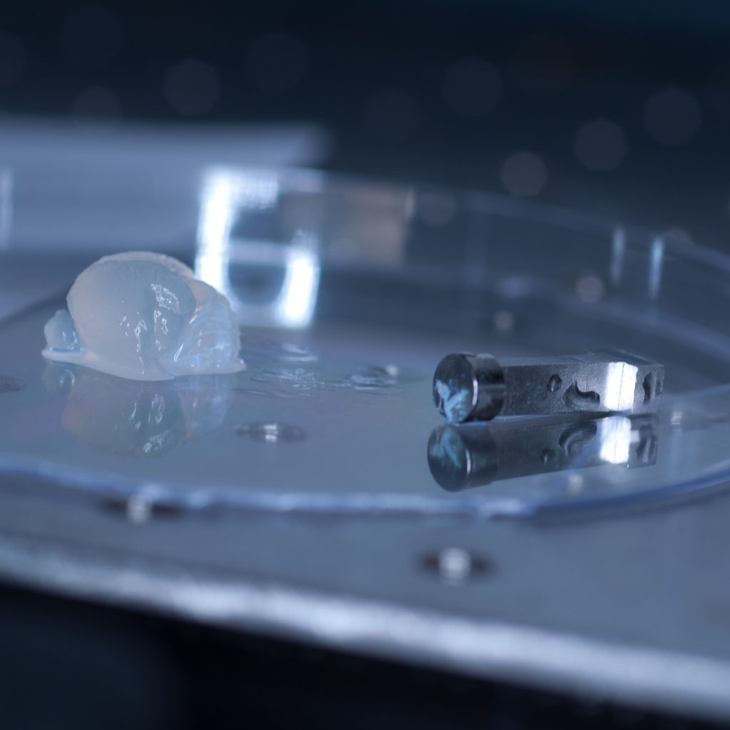
The test sample we received in PBS had been processed  by a colleague using the X-CLARITY system using standard methodologies recommended by the manufacturer. The tissue was completely transparent  after clearing, however its transferal to PBS (e.g. for post-clearing immuno-labelling) resulted in a marked change in opacity, the tissue becoming cloudy white in appearance. We thus returned the sample to distilled water (overnight at 4oC) and observed a return to optical clarity with slight osmotic swelling of the tissue.

Above: The cleared sample has a translucent, jelly-like appearance.

Generally, cleared tissue has a higher refractive index than water (n=1.33) and  X-CLARITY tissue clearing results in a refractive index close to 1.45. To avoid introducing optical aberrations that can limit resolution,  RI-matching of substrates and optics is recommended.  Consequently, our plan was to transfer the cleared tissue into X-CLARITY RI-matched (n=1.45) mounting medium and set up the lightsheet microscope for imaging of cleared tissues using a low power x5 detection objective (and x5 left and right illumination objectives) which would allow us to capture a large image field. 

Prior to fitting the x5 detection objective an RI-matched spacer ring (see below) was first screwed into the detection objective mount.

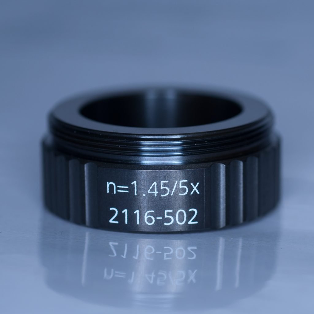
Above: Spacer ring for n=1.45 lenses.

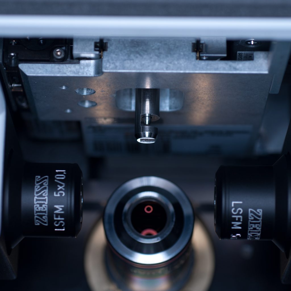
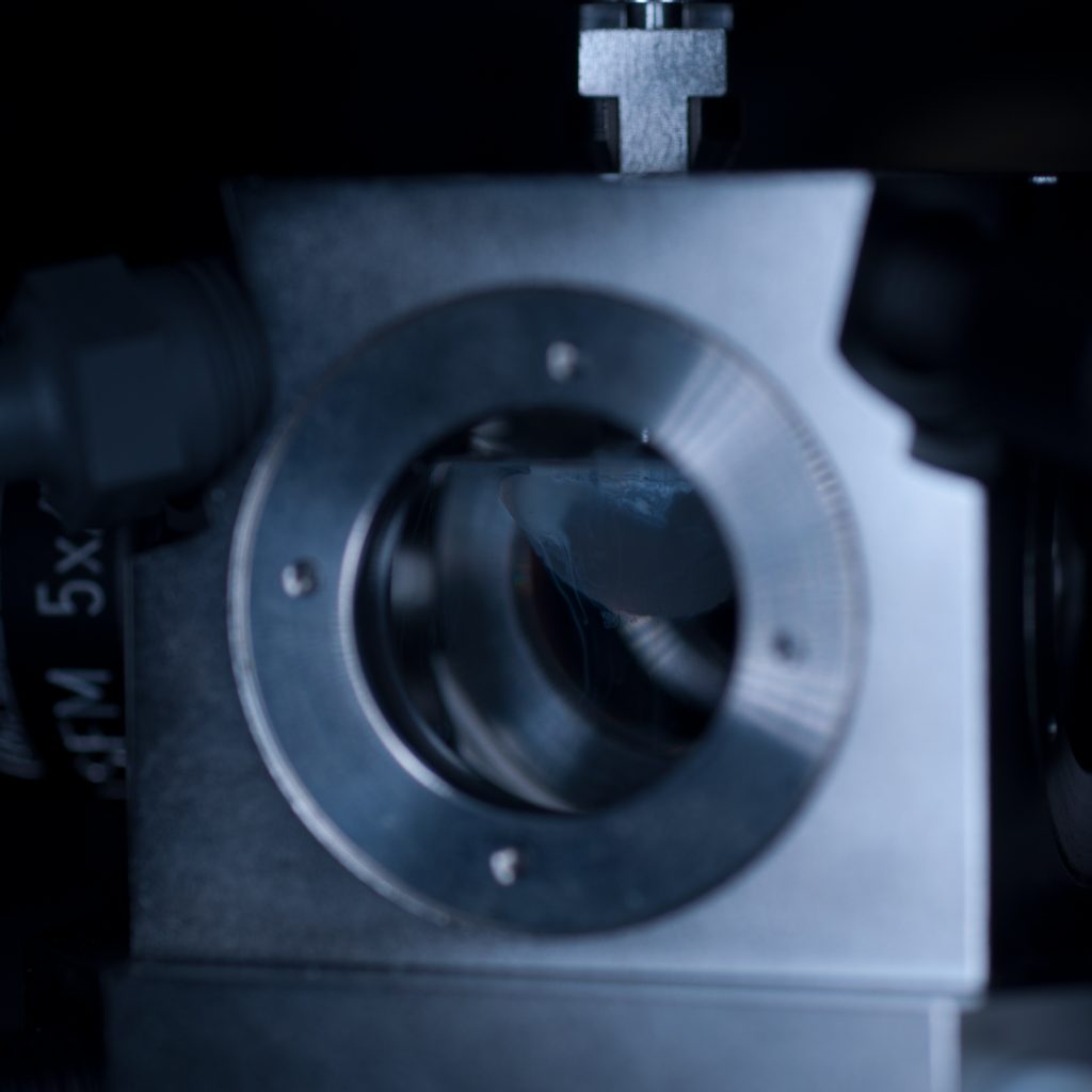
After the n=1.45 spacer ring was fitted, the x5 detection objective was screwed into place (seen centrally in below image) followed by the x5 illumination objectives to the left and right (see below).

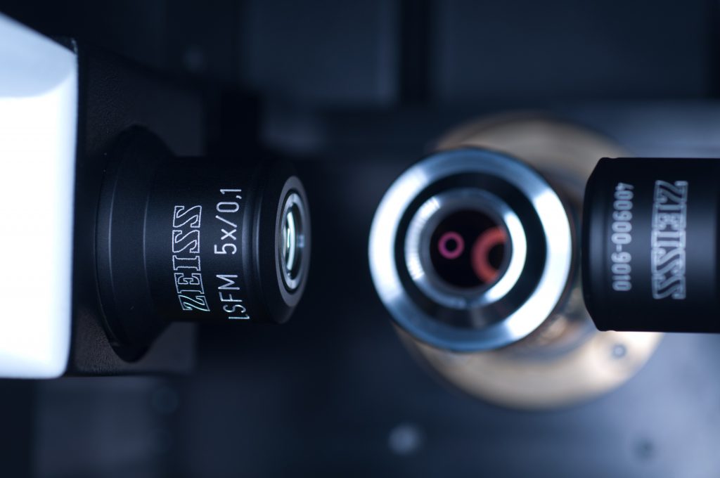
Above: Light sheet objectives. Illumination on left and right, observation to the rear.

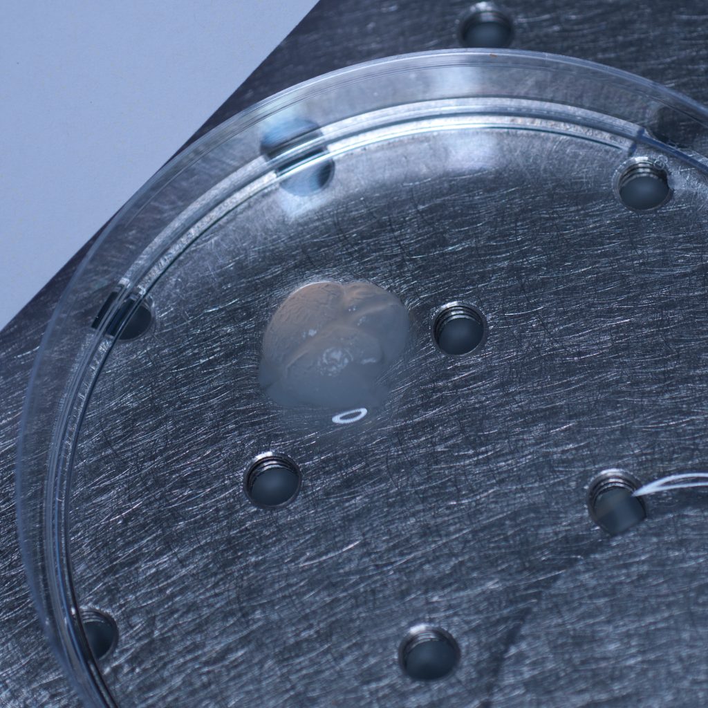
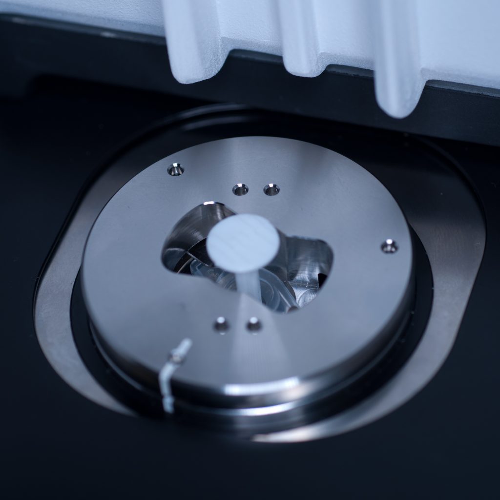
Once the objective lenses had been screwed into place, the sample chamber was inserted (see below). The use of a clearing mountant requires a specific n=1.45 sample chamber. We used the n=1.45 chamber for the x5 (air) detection objective. This chamber has glass portals (coverslips) on each of its  vertical facets (unlike the x20 clearing chamber that is open at the rear to accomodate the x20 detection lens designed for immersion observation).

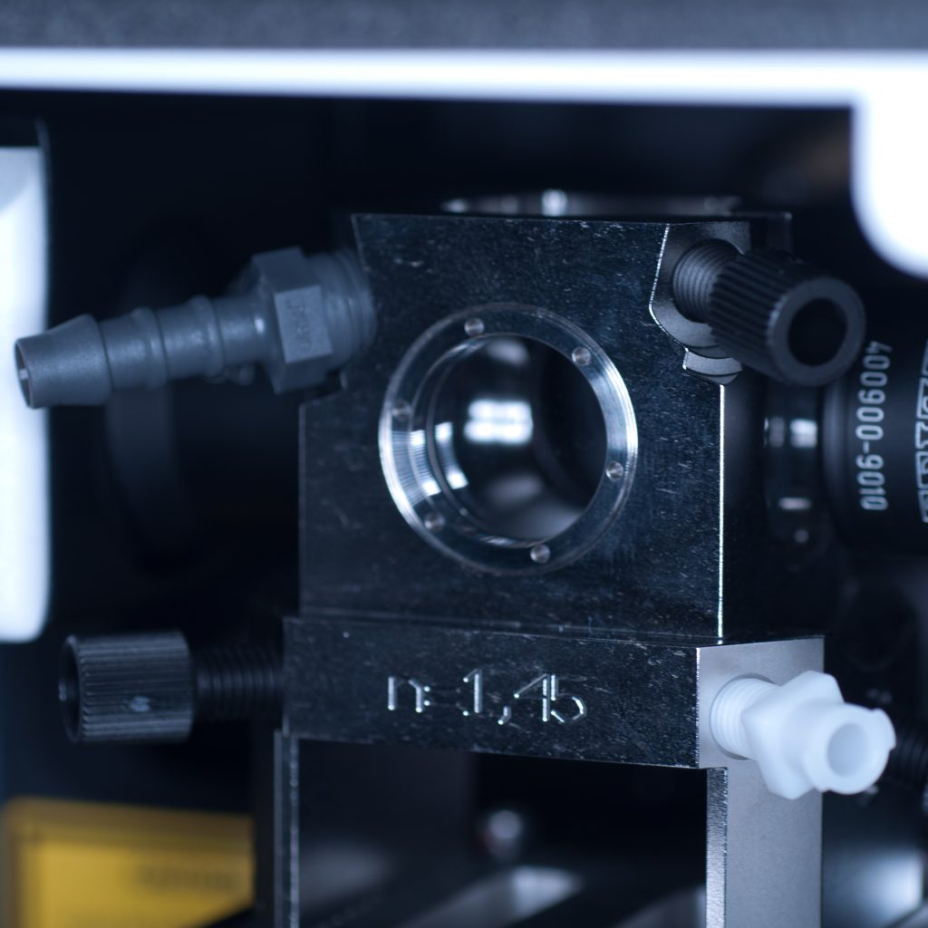
Above: Sample chamber for clearing (n=1.45).

Unfortunately, as it turned out, the RI-matched X-CLARITY mounting medium for optimum imaging of X-CLARITY cleared samples wasn’t available to us on the day, necessitating a quick re-think. As the tissue sample remained in distilled water  we decided to image, sub-optimally, in this medium. To do this we quickly swapped the n=1.45 spacer ring on the detection objective to the n=1.33 spacer. We then switched to the standard (water-based) sample chamber.

With the system set-up for imaging we set about preparing the tissue sample for presentation to the lightsheet.  As mentioned earlier, large tissue samples cannot be delivered to the sample chamber from above, as the delivery port of the specimen stage has a maximum aperture of 1cm across. This necessitates (i) removing the sample chamber (ii) introducing the specimen holder into the delivery port, (iii) manually lowering the specimen stage into place (iv) attaching the sample to the specimen holder (v) manually raising the specimen stage, (vi) re-introducing the sample chamber, and then (vii) carefully lowering the specimen into the sample chamber which can then (viii) be flooded with mounting medium.

The initial idea was to present the sample to the lightsheet, as described above, by attaching it to a 1ml plastic syringe. The syringe is introduced into the delivery port of the lightsheet via a metal sample holder disc (shown below).

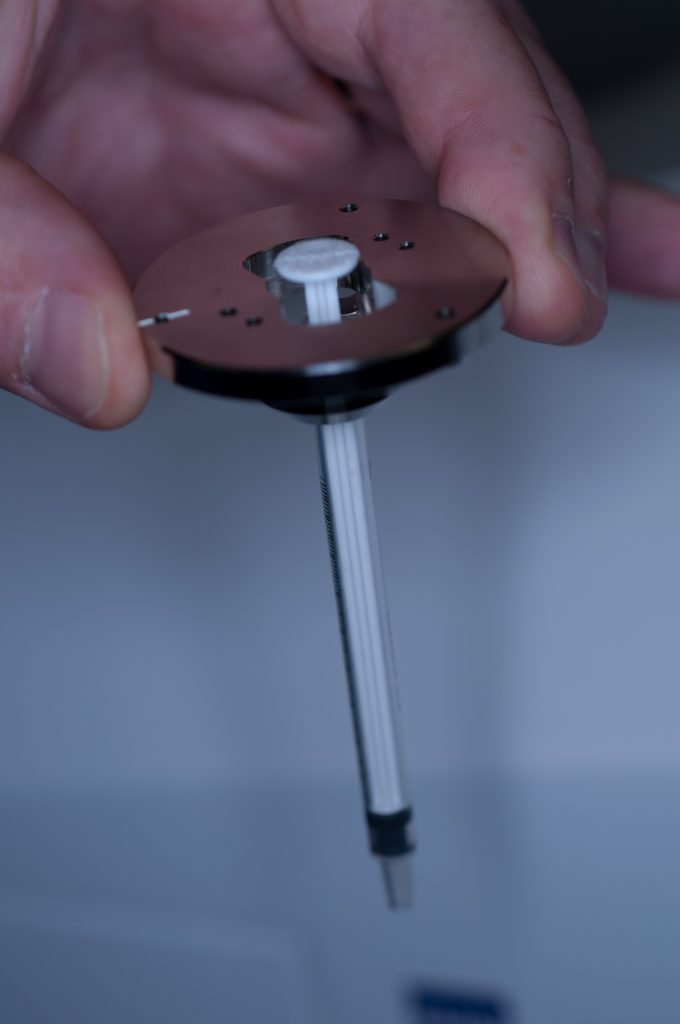
Above: Holder for 1mm syringe.

The syringe is centred in the sample holder disc via a metal adaptor collar (shown below), which must be slid along the syringe barrel all the way to its flange (finger grips). When we tried this using the BD Plastipak syringes supplied by Zeiss we found that the barrels were too thick at the base so that the the collar would not sit flush with the flange!

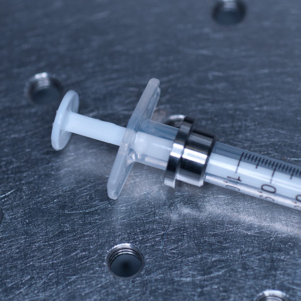
Above: Metal collar for the syringe holder.

In order to make it fit, we carefully shaved off the excess  plastic  at the base using a razor blade.

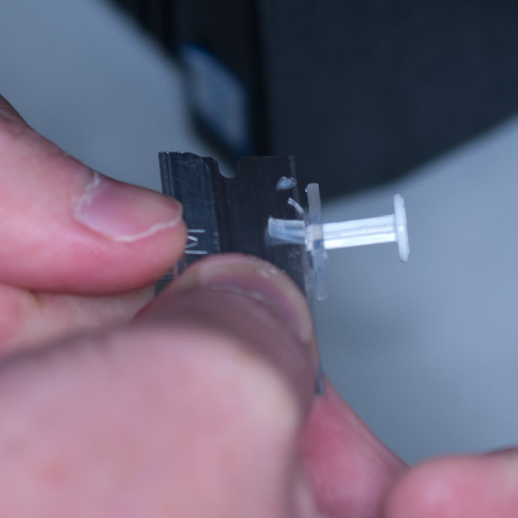
Above: Carefully shaving plastic off the syringe to make it fit.

This allowed the adaptor collar to be pushed flush against the barrel flange (see below).

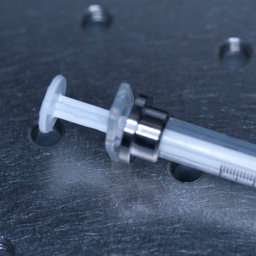
Above: Syringe with the adaptor collar in the correct position.

The flanges themselves also required a trim as they were too long to position underneath the supporting plates of the specimen holder disc. Note to self: we must find another plastic syringe supplier!

Once the syringe had been modified to correctly fit the sample holder it was introduced into the delivery port of the specimen stage, in loading position, by aligning the white markers  (see below)   

Above: Syringe plus holder inserted into the delivery port of the sample stage (note correct alignment of white markers).

With the front entrance of the lightsheet open and the sample chamber removed, the stage could be safely lowered via the manual stage controller with the safety interlock button depressed (see below). 

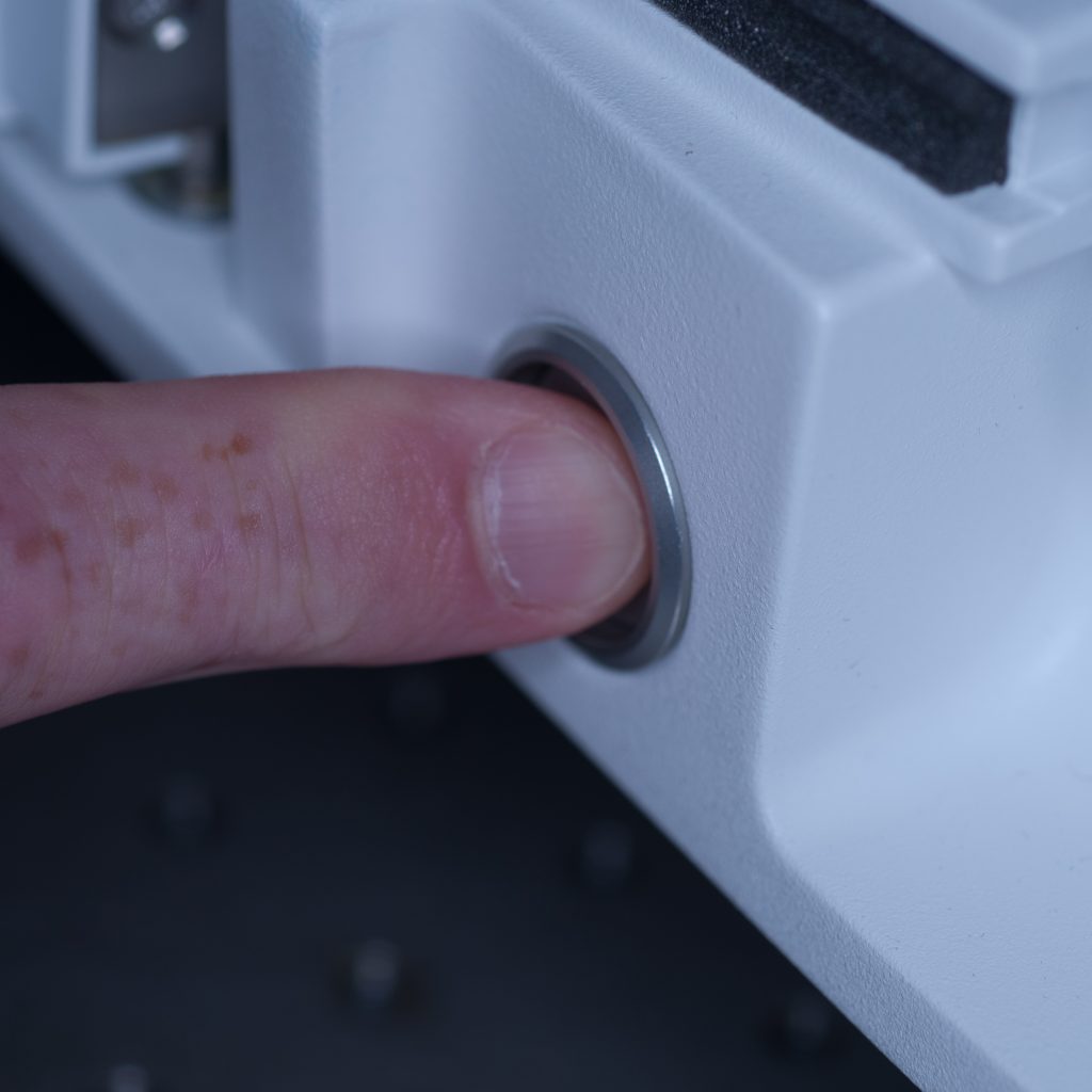
Above: Button for safety interlock under the chamber door.

The stage was lowered so that the syringe tip was accessible from the front entrance of the lightsheet (see below).

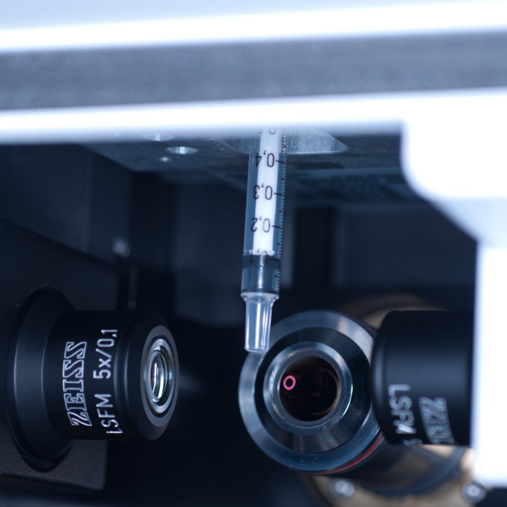
Above: Syringe dropped down to an accessible position.

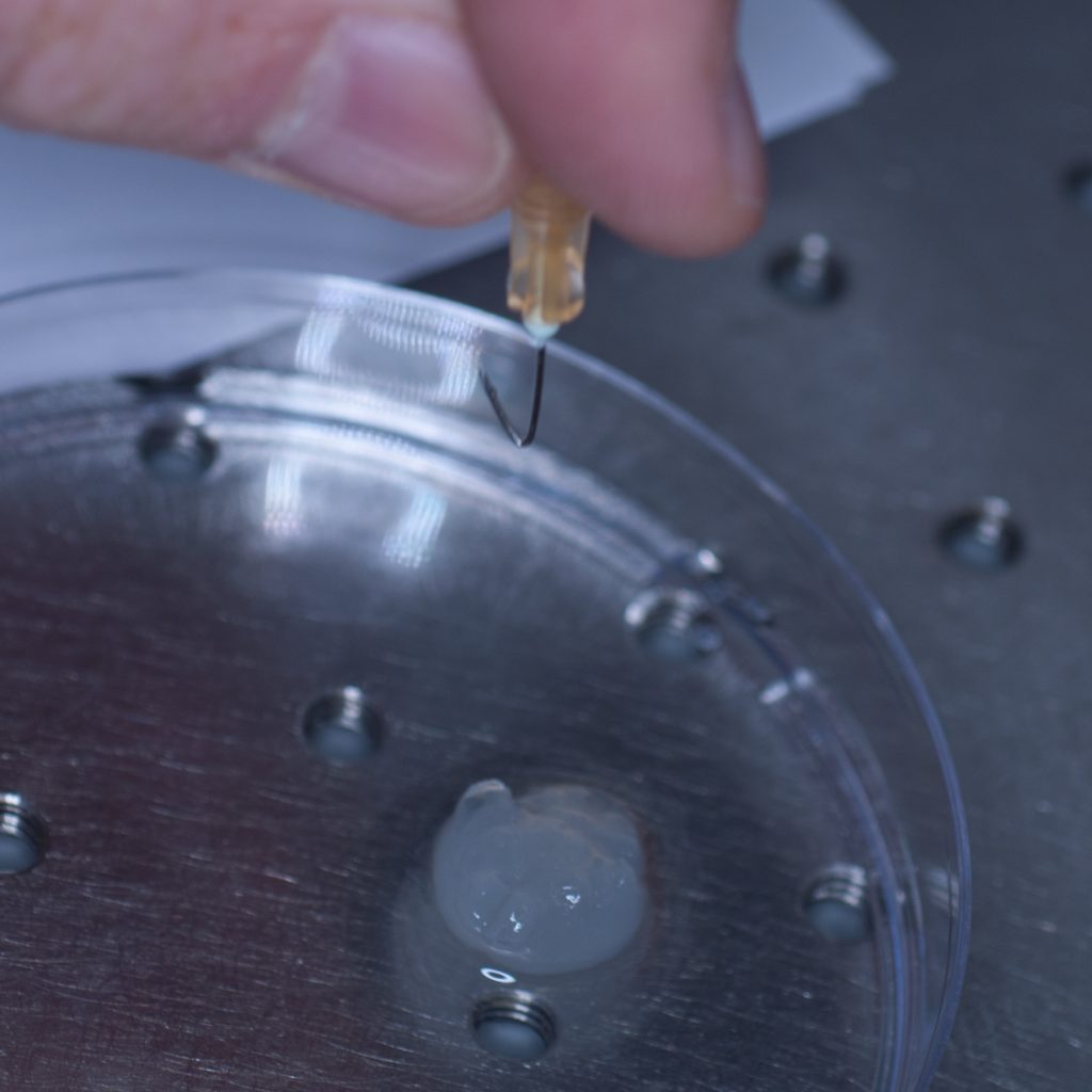
Our first thought was to impale the tissue sample onto a syringe needle so that it could then be attached to the tip of the syringe (see below).

Above: Using a needle to impale the sample.

However, this approach failed miserably as the sample slid off the needle under its own weight.  In an attempt to resolve this problem, a hook was fashioned from the needle in the hope that this would support the weight of the tissue (see below).

Above: A pair of pliers was used to bend the needle and make a hook.

Unfortunately, this approach also failed, as the hook tore through the soft tissue like a hot knife through butter.

We decided therefore to chemically bond the tissue to one of the short adaptor stubs included with the lightsheet system with super-glue. The adaptor stubs can be used with the standard sample holder stem designed for capillary insertion. They attach to the base of the stem via an internal locking rod with screw mechanism (shown below).

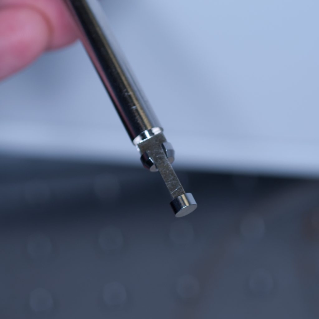
Above: Sample stub for glued samples.

To introduce the sample holder stem into the sample chamber (see below) we used essentially the same process as that described above for the syringe.

Above: The sample holder stem being  lowered into position (the central locking rod can be seen protruding out)

The tissue sample was carefully super-glued on to the adaptor stub for mounting onto the sample holder stem.

Above: Super-gluing the sample on to the adaptor stub.

Again, under its own weight, the sample tore off the stub leaving some adherent surface tissue behind (see below)

Above: Adaptor stub with tissue torn off.

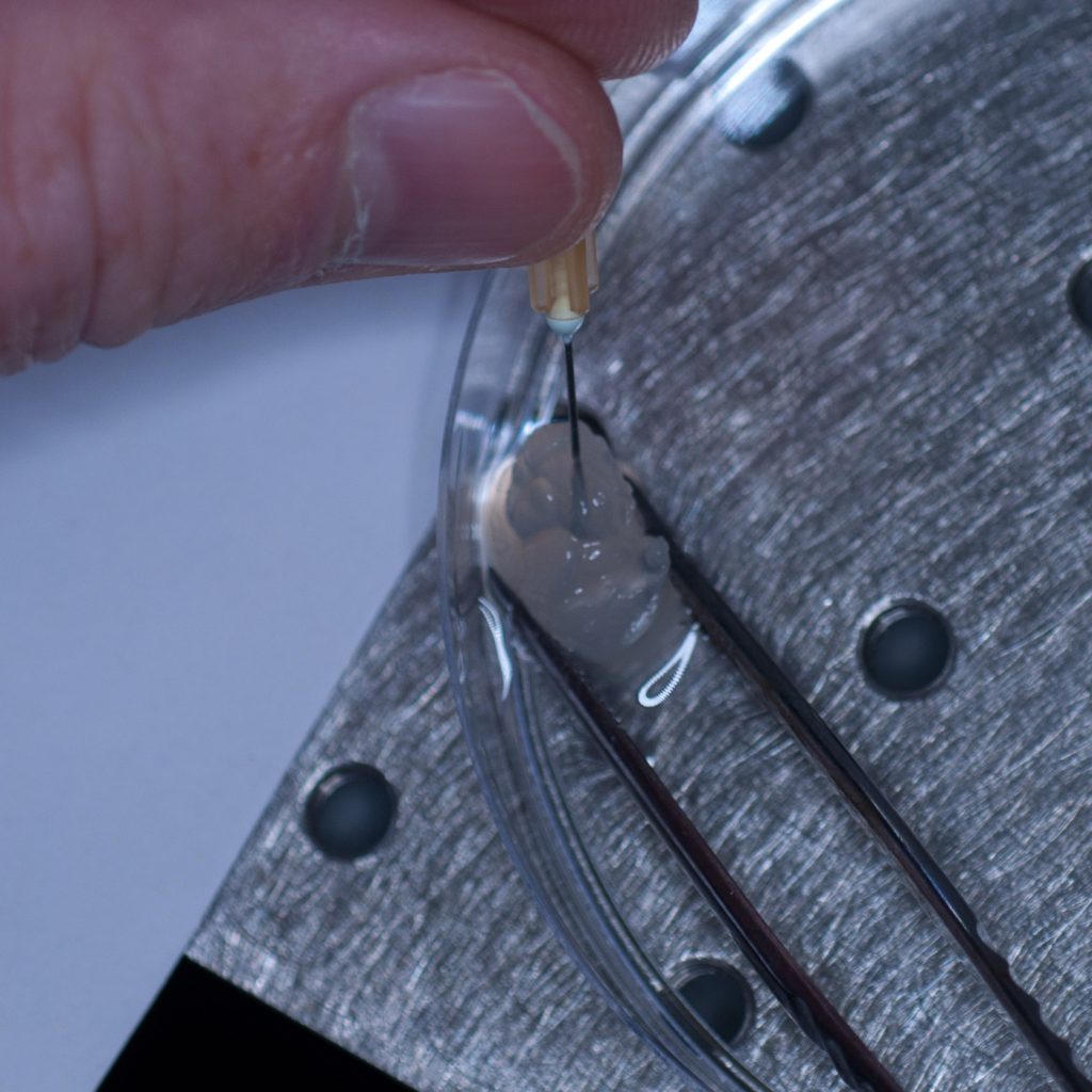
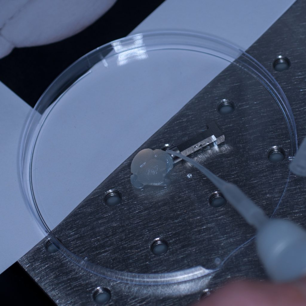
It seemed pertinent at this stage to reduce the sample volume as  it was clearly the weight of the tissue that was causing it to detach. Having already visualised the sample under epifluorescence using a stereo zoom microscope we had a very good idea of where the fluorescent signal was localised in the tissue. Consequently, we  reduced the sample to approximately one third of its original size and again glued it to the sample stub ensuring that the region of interest would be accessible to the lightsheet (see below).

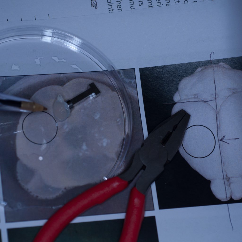
Above: Sample cut down to size and attached successfully to stub.

This time it held. The adaptor stub was then carefully secured to the sample holder stem via its locking rod, the stage manually raised  and the sample chamber introduced into the lightsheet. The sample was manually lowered  into position so that it was visible through the front viewing portal of the sample chamber. The sample chamber was then carefully filled with distilled water for imaging (remember, we didn’t have any X-CLARITY mounting medium at this stage).

Above: Sample positioned in the imaging chamber.

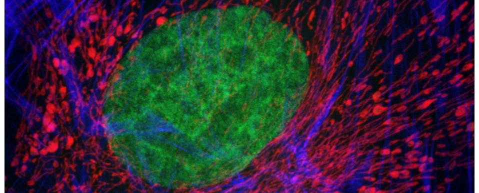
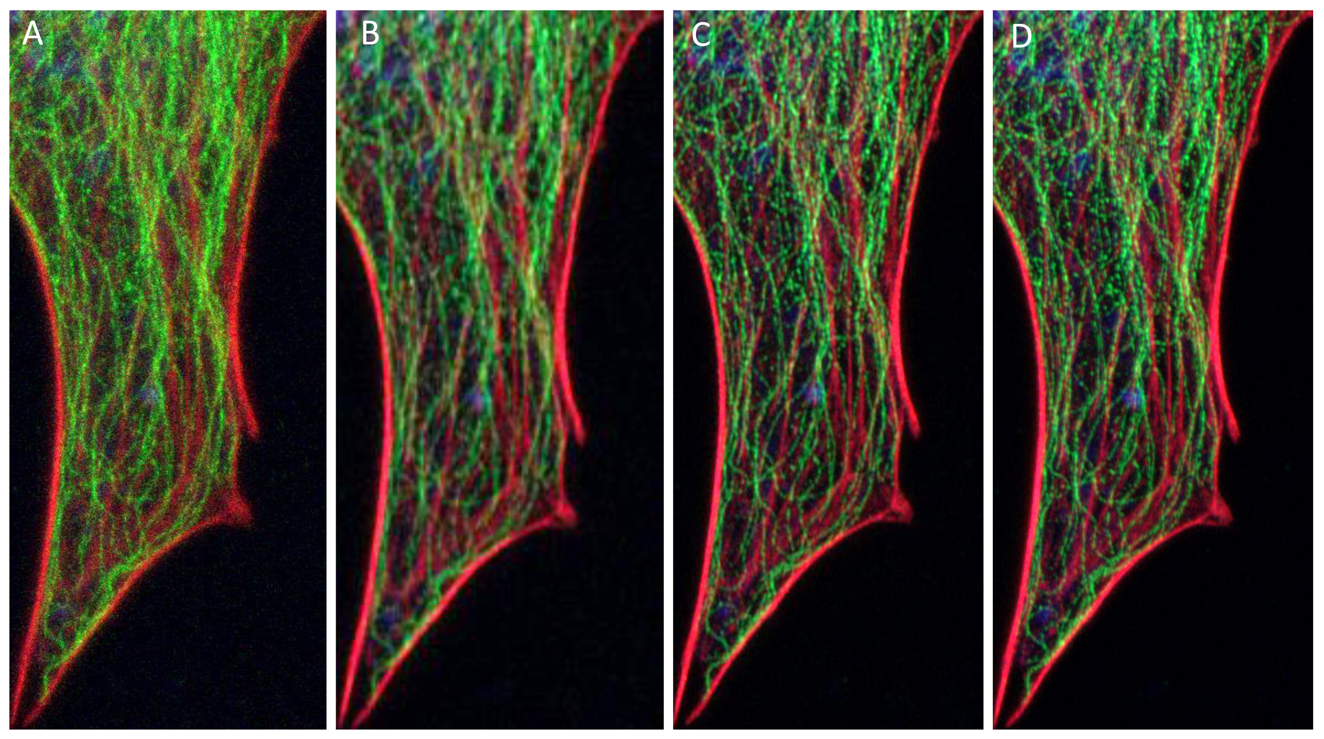
With the sample in place, we then set up the lightsheet for imaging GFP fluorescence. Due to the large sample size, we found that we could only image from one side (the lightsheet couldn’t penetrate the entire sample without being scattered or attenuated). The sample was therefore re-oriented so that the region of interest was presented directly to the lightsheet channel coming in from the right. We then switched on the pivot scan to remove any shadow artefacts and set up a few z-series through the tissue. The image below shows the sort of resolution we was getting off the x5 detection objective using maximum zoom.

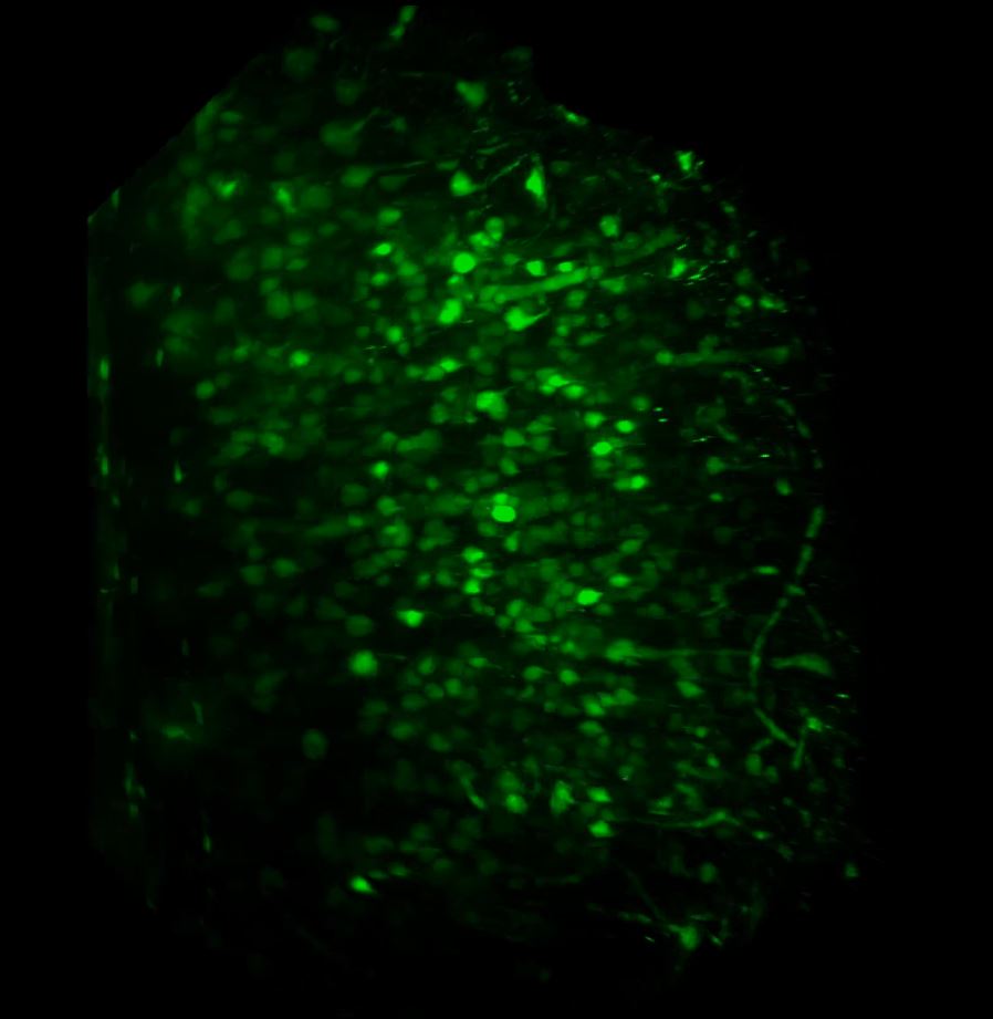
Above: Low power reconstruction of neuronal cell bodies in brain tissue. Dataset taken to a depth of 815 microns from the tissue surface  (snapshot of 3D animation sequence).

It took us a fair amount of time to establish a workflow for the correct preparation and presentation of the sample to the lightsheet.  However, once we had established this we were able to get some pretty good datasets and in very good time – the actual imaging part was relatively straightforward. The next step will be to repeat the above using the refractive-index matched X-CLARITY mounting medium,  try out the x20 clearing objective and utilise the multi-position acquisition feature of the software.

Contributions:

Tissue clearing and labelling, I. M. Garay; preparation, presentation and lightsheet imaging of sample, A. J. Hayes; photography, M. Isaacs; text, M. Isaacs and A.J.Hayes.

Further reading:


IN-FOCUS: Making Imaris a Bit(plane) Faster

Most of the work of the Bioimaging Hub is concentrated on acquiring images – choosing the right equipment, optimising settings, advising about sample prep, etc. We do, however, have a few systems dedicated to analysing images too. We’ve got a system running Arivis Vision4D which specialises in extremely large datasets, such as Lightsheet data, as well as a system running Bitplane Imaris. We’ve had Imaris for longer and so it’s seen a lot more use. This was recently updated with a Filament Tracer module for analysing neuronal processes. Shortly after this upgrade was added we experienced a severe slowdown in the software. It would take over a minute to go from the ‘Surpass’ view, where images are analysed, to the ‘Arena’ view, where files are organised. The information for the files in Arena is stored in a database and we suspected that the database was at fault.

Imaris hanging when switching from Surpass to Arena. It would do this for about 65 seconds every time a change was made.

A call with Imaris technical support was arranged and the software examined. There were no apparent errors in any of the logs and the database was functioning as it should. The only advice available was to thin down the number of entries in the database – we were told it had nearly 240,000 entries which, even accounting for metadata, seemed vastly excessive for the number of files in Arena.

Complete database dump of nearly 240,000 entries.

I decided to try to trim the database.

My first thought was the Filament Tracer module was generating a large amount of statistics and these were being stored in the database. A couple of users had been experiencing crashes when accessing these statistics so it was possible that slow database responses were bringing the software down. I backed up all datasets which used the Filament Tracer (a process far more laborious than it should be) and deleted them all from Arena. This dropped the database access time from 65 seconds to 60. Not that much of a result.

My next thought was that the co-ordinates for the vertices of surface renders might have been clogging up the database. We’ve generated quite a lot of 3D models of pollen grains and cells so this was potentially a lot of data. I went through the same laborious process of exporting all these datasets and deleted them. Again, little improvement.

I decided I needed to look at the database directly. The underlying database runs on PostgreSQL as part of the BisQue bioimaging package. Using the pgAdmin tool I began to browse the database to see where the data was held and how it was organised.

Structure of the underlying database.

I couldn’t find any trace of it so I exported the entire thing as a text file and loaded it into NotePad++. As Imaris technical support had told us, it was enormous – 55MB of text. Scanning the file, eventually I found that practically all the data was held in a database table named ‘taggable’. I’d skipped over this at first as the name was so nondescript.

Using Notepad++ to check a database dump and find where the data is stored – the table named ‘taggable’.

Once I knew all the data I needed was in this table I began to examine it. The first thing that jumped out at me was the huge number of entries in the database relating to datasets from our Leica confocal system. This system stores its data as a series of tif images, one per channel, one per z-position for z-stacks. Every single one of these files had its own database entry as a dependency for a ‘resource_parent_id’.

Database entries for Leica datasets. One record per channel, per z-position which becomes a huge number of entries.

A lot of old Leica datasets had been loaded into Arena recently to see if any new information could be extracted from them and this had massively inflated the size of the database. I exported all these datasets as new Imaris .ims files and deleted them from Arena. This reduced the number of database entries from just under 240,000 to just over 16,000. As a result the database access time dropped to about 18 seconds. Much more manageable but still a bit slow.

Looking at the database entries again, I could see that there were still lots of entries relating to Leica datasets. I went back to look at Arena but there was no sign of them. These were orphaned entries relating to non-existent data. As it was impossible to delete them from Arena, I identified all of their resource_parent_id numbers and used pgAdmin to delete them

Manually deleting orphaned database entries.

It then occurred to me that the indexes for the database were probably totally out of date so my final task to optimise things was the rebuild all of the indexes in pgAdmin

Rebuilding the table indexes.

All of these steps got the database access time down to 3 seconds – quite a bit improvement on the original 65 seconds! Importing some of the exported datasets as Imaris .ims files slowed it back down to about 10 seconds so it’s apparent that the database scales very poorly. Still a lot better than when the Leica datasets were numerous separate files though. It looks to me that the database design favours flexibility over scaling which ends up being not very useful if you want to use it to organise a reasonable amount of imaging data.

So if you’ve got Imaris database lag there’s a few things you can try. The main improvement was to make sure your datasets are represented by single files, either by exporting them as Imaris .ims files or converting them to something like OME-TIFF first.


Marc Isaacs, Bioimaging Technician

SPOKE EQUIPMENT: X-Clarity Tissue Clearing System.

One of the problems associated with imaging fluorescence in large biological samples is the obscuring effects of light scatter. Traditionally this has meant physically sectioning the material into optically-thin slices in order to visualise microscopic structure.  With the advent of new volumetric imaging techniques, e.g.  lightsheet microscopy, there is increasing demand for procedures that allow deeper interrogation of biological tissues. With this in mind, an innovative clearing system has recently been purchased through generous donations to the European Cancer Stem Cell Research Institute (ECSCRI). The equipment, which will be housed in ECSCRI lab space, allows large, intact histological samples to be rendered transparent for fluorescent labelling and 3D visualisation by confocal and lightsheet microscopy.

The X-Clarity tissue clearing system is designed to simplify, standardise and accelerate tissue clearing using the CLARITY technique (an acronymn for Clear Lipid-exchanged Acrylamide-hydridized Rigid Imaging/Immunostaining/in situ-hybridization-compatible Tissue hYdrogel). In the technique,  preserved tissues are first embedded in a hydrogel support matrix. The lipids are then extracted via electrophoresis to create a stable, optically transparent tissue-hydrogel hybrid that permits immunofluorescent labelling and downstream 3D imaging.

The new equipment and associated reagents will have wide relevance to many areas of research in Cardiff,  including deep visualisation of breast cancer tumours by Professor Matt Smalley’s research group  using  the Bioimaging Hub’s new lightsheet system. You can see a video here that shows the power of the  CLARITY technique for high resolution 3D visualisation  of tissue and organ structure.

Further Reading

AJH

CORE EQUIPMENT: Fast Module Upgrade for the Zeiss LSM880 Airyscan Confocal Microscope.

Above: Maximum intensity projections of actin stress fibres (red) and microtubules (green) of an endothelial cell imaged on a Zeiss LSM880 Airyscan confocal microscope. Z-stacks were sampled via: A. Conventional confocal optics (5 minutes scan time) B. Airyscan Fast – 0.5x Nyquist sampling (30 seconds scan time) C. Airyscan Fast – 1.5x Nyquist sampling (1 minute scan time) D. Airyscan Fast – 2x Nyquist sampling (5 mins scan time).

Through generous support of Cardiff School of Biosciences, the Bioimaging Research Hub has recently upgraded its Zeiss LSM880 Airyscan confocal system for fast image acquisition via the Zeiss Fast module upgrade. The Airyscan system allows imaging at a resolution  1.7x that of conventional confocal optics (find out more here) and the new fast  upgrade provides a 4x speed enhancement with improved signal to noise ratio. The technique uses  beam shaping optics to elongate the excitation spot along the y axis so that it simultaneously covers four lines in a single scan. This parallelisation approach, whilst increasing acquisition speeds by a factor of four, allows high pixel dwell times to be maintained resulting in high a signal to noise ratio.  You can read more about the technique below or, if you would prefer,  kick back and watch this explanatory webinar courtesy of Zeiss.

Further reading

Huff, J. (2016) The Fast mode for Zeiss LSM880 with AIryscan: high-speed confocal imaging with super-resolution and improved signal to noise. Nature Methods 13: 10.1038/nmeth.f.398.

AJH